
Issue #010: SQL and Relational Algebra — the formal foundation behind every query you've ever written
SQL looks like English. Underneath it is mathematics. Understanding the math is what separates engineers who write queries from engineers

A senior engineer at a fintech company spent two days debugging a reporting discrepancy. Their query looked right. The table had data. The filters made sense. But the result was consistently empty. No error. No warning. Just zero rows.
The query was this:
SELECT name FROM customers
WHERE region_id NOT IN (
    SELECT region_id FROM regions WHERE active = false
);
One region had a NULL in region_id. That single NULL made the entire NOT IN clause evaluate to UNKNOWN for every customer row — returning nothing. Two days of debugging for one NULL in a subquery that nobody knew was there.
This isn’t a bug. It’s the mathematically correct behaviour of SQL’s three-valued logic — a direct consequence of how NULL is defined in relational algebra. The engineer didn’t have a query problem. They had a knowledge gap: they’d learned SQL syntax without the algebra underneath it.
That algebra is what this issue covers. Not because you need to write mathematical notation — you don’t. But because when you understand the six operations that SQL is built from, queries become transparent. You’ll see immediately why that NOT IN query returns nothing, why the planner moves your WHERE clause before the JOIN, and why some “optimisations” your colleagues suggest are algebraically guaranteed to give the same result.
What relational algebra actually is
CODD didn’t design SQL. He designed the relational algebra — a set of six operations on relations (tables) that can express any fact retrievable from relational data. SQL was designed later as a human-readable syntax that maps onto those operations.
The six operations are:
σ (sigma) — Selection. Filter rows based on a predicate. σ_salary > 80000 (employee) is every row where salary exceeds 80,000. In SQL: WHERE salary > 80000.
π (pi) — Projection. Choose which columns to include. π_name, salary (employee) returns only name and salary. In SQL: SELECT name, salary.
⋈ — Join. Combine two relations on a matching condition. In SQL: JOIN ... ON.
∪ — Union. Combine two result sets with identical schemas. In SQL: UNION.
− — Difference. Rows in one relation that don’t appear in another. In SQL: EXCEPT.
ρ (rho) — Rename. Give a relation or attribute a new name. In SQL: AS.
That’s the complete vocabulary. Every SQL query you’ve ever written — no matter how complex, with subqueries, CTEs, window functions, and recursive joins — is a composition of these six operations. The query planner translates your SQL into an algebra tree and then finds the most efficient physical execution of that tree.
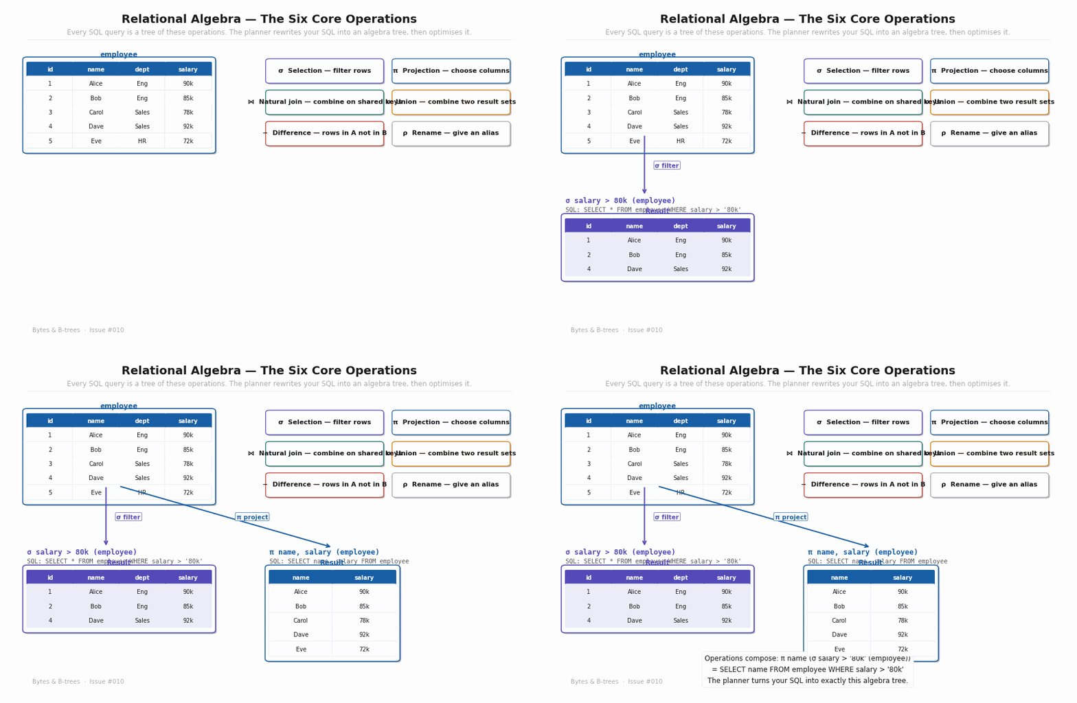
The diagram shows each operation applied to an employee table, with results appearing alongside. The key observation in the last stage: operations compose. π name (σ salary > 80000 (employee)) applies selection first, then projection — which is exactly what SELECT name FROM employee WHERE salary > 80000 does. The planner sees your SQL, builds this algebra expression, and then decides whether to apply the selection before or after loading the full table.
Why the algebra explains query optimisation
Here is the insight that makes database query planning make sense: algebraic equivalences let the planner legally rewrite your query into a faster form.
Two algebra expressions are equivalent if they always produce the same result on any valid input. The planner maintains a library of these equivalences — hundreds of rewrite rules — and applies them before choosing a physical execution strategy.
The most important one for everyday SQL:
Selection pushdown: σ_condition(R ⋈ S) is equivalent to σ_condition(R) ⋈ S
In English: filtering rows before joining is mathematically the same as filtering rows after joining — but filtering first means fewer rows enter the join, making the join dramatically cheaper.
This is why the planner moves WHERE clauses before JOIN operations. Not as a heuristic. Not as a “best practice.” As an algebraic guarantee. The result is identical either way, and one path is faster.
Other equivalences the planner applies:
-- These two queries are algebraically identical:
SELECT * FROM orders WHERE status = 'shipped' AND amount > 100;
SELECT * FROM orders WHERE amount > 100 AND status = 'shipped';
-- Predicate order in WHERE is irrelevant. Planner reorders for index use.

-- These are also equivalent:
SELECT DISTINCT customer_id FROM orders;
SELECT customer_id FROM orders GROUP BY customer_id;
-- Both express π with duplicate elimination. Planner may choose either plan.

-- Subquery to join rewrite (planner does this automatically):
SELECT name FROM customers
WHERE id IN (SELECT customer_id FROM orders WHERE amount > 500);
-- Equivalent to:
SELECT DISTINCT c.name FROM customers c
JOIN orders o ON c.id = o.customer_id
WHERE o.amount > 500;
When you understand that these rewrites are algebraic equivalences — not approximations — you stop worrying whether the planner will “do the right thing.” It will, because the right thing is mathematically defined.
The fundamental unit of relational algebra: the relation
A relation is not just “a table.” Formally, a relation is a set of tuples — and sets have no duplicates and no ordering. These two properties have direct SQL consequences:
No ordering: A bare SELECT has no guaranteed row order. This surprises engineers who see consistent ordering in testing and assume it’s guaranteed. It isn’t. Without ORDER BY, a query can return rows in any order the planner chooses — and that order can change when you add an index, update statistics, or upgrade Postgres. Always use ORDER BY when order matters.
No duplicates: A true relation has no duplicate rows. SQL allows duplicates (it’s a multiset, technically) — which is why SELECT DISTINCT exists, and why CODD’s Rule 12 is violated by SQL at a theoretical level. For most practical purposes this doesn’t matter. For queries that depend on set semantics (UNION vs UNION ALL, EXCEPT vs EXCEPT ALL), it matters significantly.
How the query lifecycle uses algebra
Every SQL query passes through this pipeline before a single row is read:
1. Parse — Your SQL string is tokenised and parsed into a parse tree. Syntax errors are caught here.
2. Analyse — Names are resolved: employee → relation OID 16385, salary → attribute 4 of that relation. Type checking happens. Semantic errors are caught here.
3. Rewrite — View definitions are inlined. Rule-based rewrites are applied. If your query references a view, the view’s definition is substituted into the query tree here.
4. Plan (logical) — The parse tree is converted into a logical algebra tree. Equivalence rewrites are applied — selection pushdown, join reordering, subquery flattening. The planner generates multiple candidate trees.
5. Plan (physical) — Each logical algebra operation is assigned a physical implementation: should this join use hash join, merge join, or nested loop? Should this selection use an index scan or sequential scan? Should this sort use an explicit sort node or an index scan that returns rows pre-sorted? The planner estimates costs using table statistics and picks the cheapest physical plan.
6. Execute — The physical plan runs. Rows are returned.
Steps 4 and 5 are where the algebra matters. The planner can only rewrite the logical tree safely because the rewrites are algebraic equivalences. If they weren’t, the planner would need to ask you for permission before each rewrite — and SQL would be far less usable.
Try this right now
Run this on any Postgres database with data:
EXPLAIN (FORMAT TEXT)
SELECT e.name, d.dept_name
FROM   employee e
JOIN   department d ON e.dept_id = d.id
WHERE  e.salary > 80000;
Look at the output. Find the line that says Filter: (salary > 80000). Note whether that filter appears above or below the join node. In almost every case, Postgres will have pushed the filter below the join — applying it to the employee table before the join happens.
Now try:
EXPLAIN (FORMAT TEXT)
SELECT e.name, d.dept_name
FROM   (SELECT * FROM employee WHERE salary > 80000) e
JOIN   department d ON e.dept_id = d.id;
Compare the plans. They’re identical. Postgres recognises that both SQL forms produce the same algebra tree after selection pushdown — and generates the same plan for both. That’s the algebra at work.
The paid section explains what the other nodes in this plan mean, how to read the cost estimates, and — importantly — the three cases where Postgres cannot push selection below a join, why, and how to rewrite your query to help it.
What’s in this issue’s paid section
✦ Three-valued logic and NULL — the complete truth tables with every trap explained
✦ The SQL algebra tree diagram — how Postgres builds and rewrites your query plan
✦ The five equivalence rules you can apply yourself to rewrite slow queries
✦ When selection pushdown fails — three cases and how to fix them
✦ Full hands-on experiments: query equivalences, NULL behaviour, EXPLAIN analysis
✦ Production checklist: 7 NULL-related bugs to audit in your existing queries
✦ Query Lab annotated solution from Issue #009
✦ Downloadable cheat sheet: SQL ↔ relational algebra reference card$15/month · $120/year · cancel anytime Subscribe → bytesandbrees.substack.com
Three-valued logic — where the fintech bug lives
SQL has three truth values: TRUE, FALSE, and UNKNOWN. UNKNOWN arises whenever NULL is involved in a comparison. This isn’t a Postgres quirk — it’s the formal definition of NULL in relational theory, designed to represent “unknown or inapplicable information.”
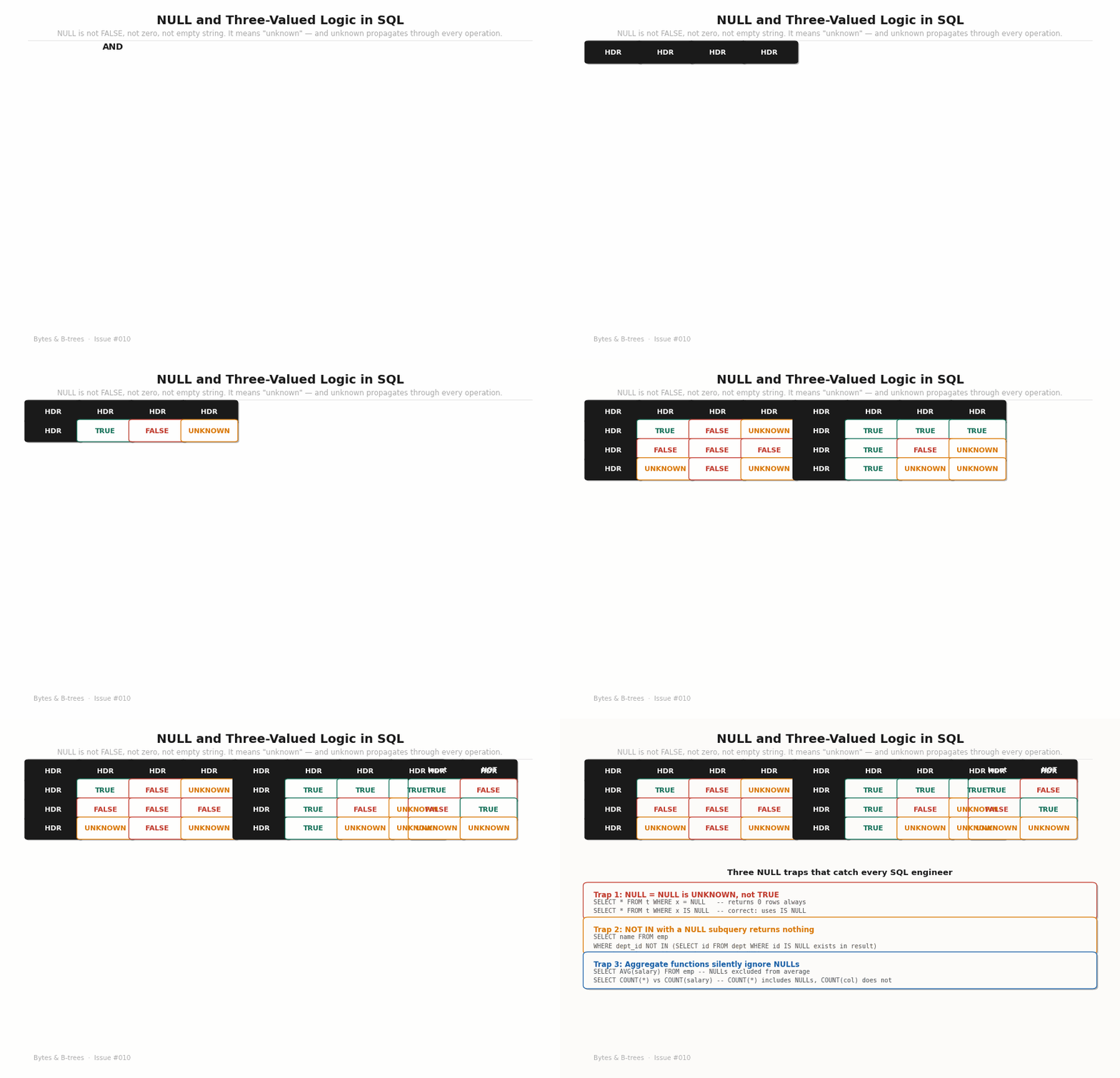
The diagram builds the AND, OR, and NOT truth tables for three-valued logic, then reveals the three traps in sequence.
The AND table has one surprising entry: FALSE AND UNKNOWN = FALSE. Why? Because regardless of what UNKNOWN resolves to (true or false), anding with FALSE gives FALSE. So FALSE AND UNKNOWN is definitely FALSE. But TRUE AND UNKNOWN = UNKNOWN — because if the unknown part turns out to be false, the whole expression is false.
The OR table has the symmetric surprising entry: TRUE OR UNKNOWN = TRUE. Because regardless of what UNKNOWN resolves to, oring with TRUE gives TRUE.
These rules are internally consistent and mathematically correct. They’re also the source of bugs that have been in production codebases for years.
Trap 1: NULL = NULL is UNKNOWN, not TRUE
SELECT * FROM orders WHERE cancelled_at = NULL;  -- always 0 rows
SELECT * FROM orders WHERE cancelled_at IS NULL;  -- correct
The equality operator applied to NULL produces UNKNOWN. SQL’s WHERE clause only returns rows where the predicate evaluates to TRUE — UNKNOWN rows are excluded, same as FALSE. IS NULL is the correct predicate; it’s a separate operator that specifically tests for null.
This trap is so common that some SQL clients warn you. Many don’t.
Trap 2: NOT IN with a NULL in the subquery
This is the bug from the opening story. Recall:
SELECT name FROM customers
WHERE region_id NOT IN (
    SELECT region_id FROM regions WHERE active = false
);
If any row in the subquery returns NULL for region_id, the NOT IN predicate evaluates to UNKNOWN for every row in customers — because:
region_id NOT IN (1, 2, NULL)
= region_id != 1 AND region_id != 2 AND region_id != NULL
= region_id != 1 AND region_id != 2 AND UNKNOWN
= UNKNOWN (for any value of region_id)
The fix: either explicitly exclude NULLs from the subquery, or use NOT EXISTS instead (which is immune to NULL):
-- Fix 1: exclude NULLs from subquery
SELECT name FROM customers
WHERE region_id NOT IN (
    SELECT region_id FROM regions
    WHERE active = false AND region_id IS NOT NULL
);

-- Fix 2: NOT EXISTS (preferred — immune to NULL, often better plan)
SELECT name FROM customers c
WHERE NOT EXISTS (
    SELECT 1 FROM regions r
    WHERE r.region_id = c.region_id
      AND r.active = false
);
The NOT EXISTS version is also frequently faster because the planner can use an anti-join, which short-circuits as soon as it finds one matching row.
Trap 3: COUNT(*) vs COUNT(column)
SELECT COUNT(*),       -- counts all rows, including NULLs
       COUNT(salary),  -- counts only non-NULL salary values
       AVG(salary)     -- NULLs excluded from average denominator
FROM employees;
If 3 of 100 employees have NULL salary, COUNT(*) returns 100, COUNT(salary) returns 97, and AVG(salary) divides by 97 — not 100. This makes AVG behave like “average salary among employees who have a recorded salary” not “average salary across all employees.” If you mean the latter, use AVG(COALESCE(salary, 0)).
The SQL algebra tree — what the planner actually builds
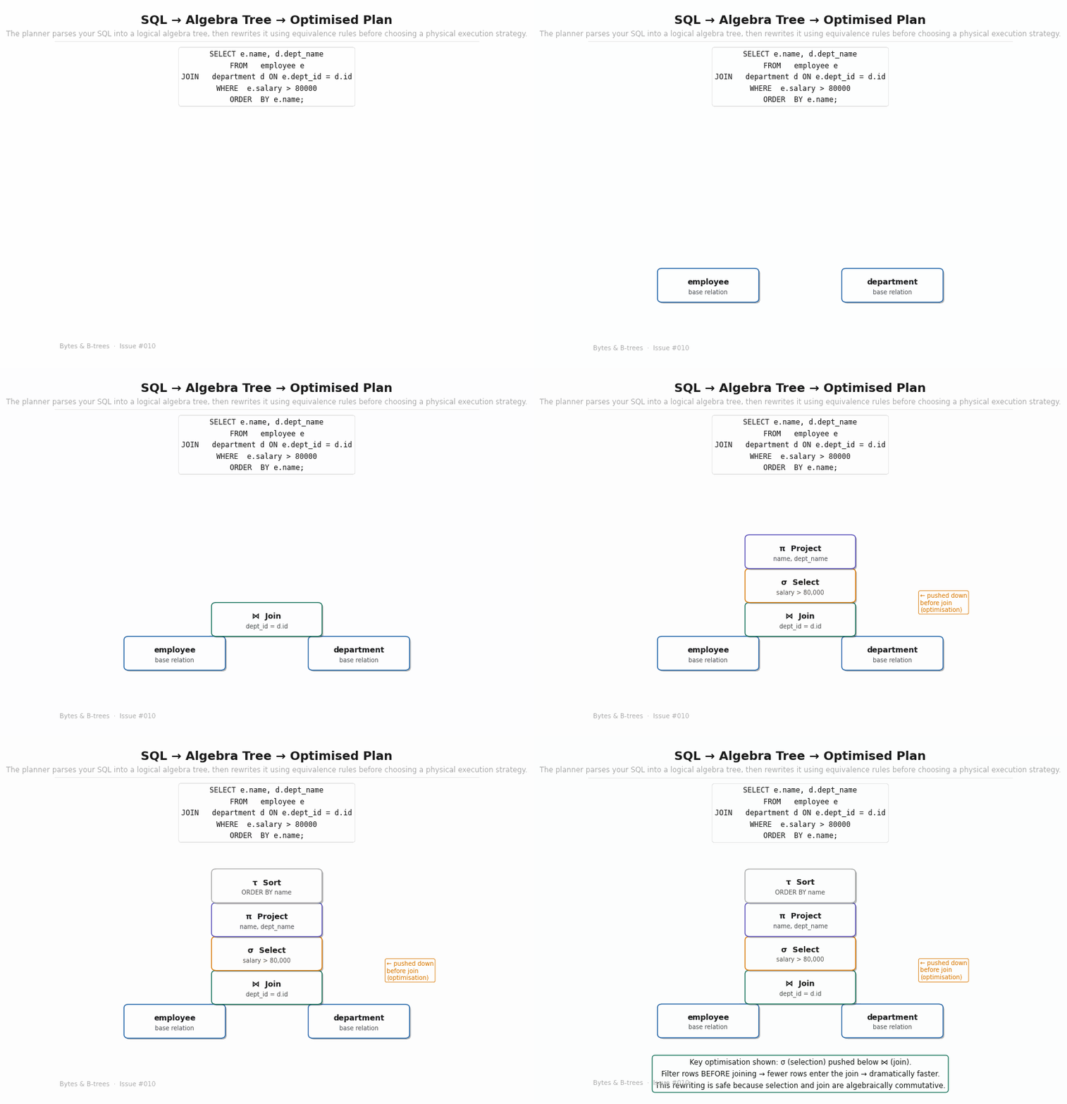
The diagram builds the algebra tree for a JOIN query with a WHERE clause and ORDER BY, one node at a time — base tables at the leaves, operations stacking toward the root. The critical annotation appears at step 3: the selection node (σ salary > 80,000) is shown at the leaves, below the join — the result of selection pushdown.
The planner builds the initial tree with selection at the top (where your WHERE clause is syntactically), then applies the pushdown rewrite. This single rewrite can make a query 10–100x faster when the filtered table is large.
Three cases where pushdown fails
The planner cannot push selection below a join in these cases:
Case 1 — The predicate references both tables:
-- Cannot push: predicate uses columns from both tables
SELECT * FROM employee e JOIN department d ON e.dept_id = d.id
WHERE e.salary > d.avg_salary;
-- The join must happen first; you can't filter on d.avg_salary before joining
Case 2 — The predicate uses a volatile function:
-- Cannot push: random() is evaluated per-row and must stay above the join
SELECT * FROM employee e JOIN department d ON e.dept_id = d.id
WHERE e.score > random() * 100;
-- If pushed below, each table side would get different random() values
Case 3 — OUTER JOIN semantics:
-- Cannot always push: LEFT JOIN null-fills right side; WHERE on right side
-- effectively converts to an INNER JOIN, which changes semantics
SELECT e.name, d.dept_name
FROM employee e LEFT JOIN department d ON e.dept_id = d.id
WHERE d.budget > 100000;
-- This already is an inner join in effect; Postgres converts it
-- But if you meant to keep employees without departments, write it differently
Understanding these cases lets you write queries that give the planner room to optimise — and lets you diagnose cases where a plan isn’t as fast as expected.
